كيفية تضمين تصورات بايثون التفاعلية على موقعك الإلكتروني باستخدام Matplotlib و mpld3

Updated يونيو 16, 2026 7 min read

Aldawsari

دقائق القراءة: 7

لقد أحدثت تصورات البيانات ثورة في طريقة فهمنا للمعلومات المعقدة. في عالم تطوير الويب، أصبح تقديم هذه التصورات بشكل تفاعلي ضرورة لتعزيز تجربة المستخدم. في مقال سابق على منصة قيد، ناقشنا كيفية إنشاء تصورات بيانات بايثون ذاتية التحديث. ولكن ماذا لو أردنا إضافة لمسة من التفاعل؟ لحسن الحظ، توجد حلول سهلة لتحقيق ذلك. في هذا الدليل الشامل، سنستكشف كيفية بناء تصورات بيانات تفاعلية باستخدام بايثون، والتي تعد مثالية للتضمين على مدونتك أو موقعك الإلكتروني.

فهم التصور البياني الذي سنعمل عليه

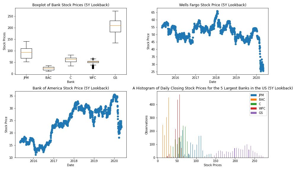
بدلاً من البدء من الصفر، سنعتمد في هذا المقال على التصور البياني الذي أنشأناه في دليلنا السابق. يستخدم هذا التصور مكتبات pandas و matplotlib في بايثون لعرض نقاط بيانات متنوعة من أكبر خمسة بنوك مدرجة علنًا في الولايات المتحدة. يمثل هذا التصور نقطة انطلاق ممتازة لإضافة ميزات التفاعل.

إليك صورة ثابتة للتصور الذي أنشأناه سابقًا:

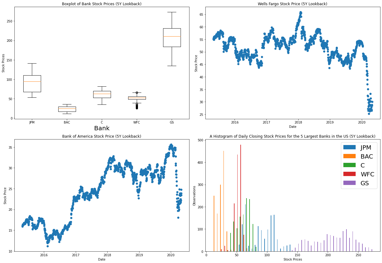
الكود الفعلي لإنشاء هذا التصور مدرج أدناه. لقد تناولنا هذا بالتفصيل في الدليل السابق، ولكن يرجى ملاحظة أنك ستحتاج إلى إنشاء مفتاح API خاص بك من IEX Cloud وتضمينه في متغير IEX_API_Key لكي يعمل السكريبت بشكل صحيح.


########################
#Import dependencies
########################
import pandas as pd
import matplotlib.pyplot as plt

########################
#Import and clean data
########################
IEX_API_Key = ''
tickers = [
    'JPM',
    'BAC',
    'C',
    'WFC',
    'GS',
]

#Create an empty string called `ticker_string` that we'll add tickers and commas to
ticker_string = ''

#Loop through every element of `tickers` and add them and a comma to ticker_string
for ticker in tickers:
    ticker_string += ticker
    ticker_string += ','

#Drop the last comma from `ticker_string`
ticker_string = ticker_string[:-1]

#Create the endpoint and years strings
endpoints = 'chart'
years = '5'

#Interpolate the endpoint strings into the HTTP_request string
HTTP_request = f'https://cloud.iexapis.com/stable/stock/market/batch?symbols={ticker_string}&types={endpoints}&range={years}y&cache=true&token={IEX_API_Key}'

#Send the HTTP request to the IEX Cloud API and store the response in a pandas DataFrame
bank_data = pd.read_json(HTTP_request)

#Create an empty list that we will append pandas Series of stock price data into
series_list = []

#Loop through each of our tickers and parse a pandas Series of their closing prices over the last 5 years
for ticker in tickers:
    series_list.append(pd.DataFrame(bank_data[ticker]['chart'])['close'])

#Add in a column of dates
series_list.append(pd.DataFrame(bank_data['JPM']['chart'])['date'])

#Copy the 'tickers' list from earlier in the script, and add a new element called 'Date'.
#These elements will be the column names of our pandas DataFrame later on.
column_names = tickers.copy()
column_names.append('Date')

#Concatenate the pandas Series togehter into a single DataFrame
bank_data = pd.concat(series_list, axis=1)

#Name the columns of the DataFrame and set the 'Date' column as the index
bank_data.columns = column_names
bank_data.set_index('Date', inplace = True)

########################
#Create the Python figure
########################
#Set the size of the matplotlib canvas
fig = plt.figure(figsize = (18, 8))

################################################
################################################
#Create subplots in Python
################################################
################################################

########################
#Subplot 1
########################
plt.subplot(2, 2, 1)

#Generate the boxplot
plt.boxplot(bank_data.transpose())

#Add titles to the chart and axes
plt.title('Boxplot of Bank Stock Prices (5Y Lookback)')
plt.xlabel('Bank')
plt.ylabel('Stock Prices')

#Add labels to each individual boxplot on the canvas
ticks = range(1, len(bank_data.columns)+1)
labels = list(bank_data.columns)
plt.xticks(ticks,labels)

########################
#Subplot 2
########################
plt.subplot(2, 2, 2)

#Create the x-axis data
dates = bank_data.index.to_series()
dates = [pd.to_datetime(d) for d in dates]

#Create the y-axis data
WFC_stock_prices = bank_data['WFC']

#Generate the scatterplot
plt.scatter(dates, WFC_stock_prices)

#Add titles to the chart and axes
plt.title("Wells Fargo Stock Price (5Y Lookback)")
plt.ylabel("Stock Price")
plt.xlabel("Date")

########################
#Subplot 3
########################
plt.subplot(2, 2, 3)

#Create the x-axis data
dates = bank_data.index.to_series()
dates = [pd.to_datetime(d) for d in dates]

#Create the y-axis data
BAC_stock_prices = bank_data['BAC']

#Generate the scatterplot
plt.scatter(dates, BAC_stock_prices)

#Add titles to the chart and axes
plt.title("Bank of America Stock Price (5Y Lookback)")
plt.ylabel("Stock Price")
plt.xlabel("Date")

########################
#Subplot 4
########################
plt.subplot(2, 2, 4)

#Generate the histogram
plt.hist(bank_data.transpose(), bins = 50)

#Add a legend to the histogram
plt.legend(bank_data.columns,fontsize=10)

#Add titles to the chart and axes
plt.title("A Histogram of Daily Closing Stock Prices for the 5 Largest Banks in the US (5Y Lookback)")
plt.ylabel("Observations")
plt.xlabel("Stock Prices")

plt.tight_layout()

################################################
#Save the figure to our local machine
################################################
plt.savefig('bank_data.png')

الآن بعد أن أصبح لدينا فهم واضح للتصور البياني الذي سنعمل عليه، دعنا نتعمق في معنى أن يكون التصور تفاعليًا.

ماذا يعني التصور البياني التفاعلي؟

هناك نوعان رئيسيان من تصورات البيانات التي يمكن تضمينها بفعالية على موقعك الإلكتروني:

التصورات الثابتة (Static Visualizations)

هذه التصورات هي في الأساس صور بسيطة، مثل ملفات .png أو .jpg. إنها تقدم لقطة واحدة للبيانات ولا تتغير استجابةً لتفاعل المستخدم.
التصورات الديناميكية (Dynamic Visualizations)

تتغير هذه التصورات وتتفاعل مع سلوك المستخدم، عادةً من خلال ميزات مثل التكبير (zooming) والتحريك (panning). لا يتم تخزين التصورات الديناميكية كملفات صور عادية، بل غالبًا ما يتم تضمينها باستخدام وسوم svg أو iframe، مما يسمح لها بالاستجابة لإدخالات المستخدم.

يركز هذا الدليل على إنشاء تصورات بيانات ديناميكية. على وجه التحديد، سيمتلك التصور الذي نسعى لإنشائه الخصائص التالية:

زر في الزاوية السفلية اليسرى لتمكين الوضع الديناميكي.
القدرة على التكبير والتحريك باستخدام الماوس بمجرد تمكين الوضع الديناميكي.
إمكانية قص جزء معين من التصور وتكبيره للتركيز عليه.

في القسم التالي، ستتعلم كيفية تثبيت واستيراد مكتبة mpld3، وهي الاعتماد البرمجي في بايثون الذي سنستخدمه لإنشاء هذه الرسوم البيانية التفاعلية.

تثبيت واستيراد مكتبة mpld3

لاستخدام مكتبة mpld3 في تطبيق بايثون الخاص بنا، نحتاج إلى إكمال خطوتين أساسيتين:

تثبيت مكتبة mpld3 على الجهاز الذي نعمل عليه.
استيراد مكتبة mpld3 إلى سكريبت بايثون الخاص بنا.

خطوات التثبيت

أسهل طريقة لتثبيت mpld3 على جهازك المحلي هي استخدام مدير الحزم pip الخاص ببايثون 3. إذا كان pip مثبتًا بالفعل على جهازك، يمكنك القيام بذلك عن طريق تشغيل الأمر التالي من سطر الأوامر:

pip3 install mpld3

استيراد المكتبة في بايثون

الآن بعد أن تم تثبيت mpld3 على جهازنا، يمكننا استيراده إلى سكريبت بايثون الخاص بنا باستخدام العبارة التالية:

import mpld3

لتحسين قابلية القراءة، يُعد تضمين هذا الاستيراد مع بقية الاستيرادات في الجزء العلوي من السكريبت ممارسة جيدة. هذا يعني أن قسم الاستيرادات الخاص بك سيبدو الآن كما يلي:


########################
#Import dependencies
########################
import pandas as pd
import matplotlib.pyplot as plt
import mpld3

تحويل تصورات Matplotlib الثابتة إلى تفاعلية

تتمثل الوظيفة الرئيسية لمكتبة mpld3 في أخذ تصور matplotlib موجود وتحويله إلى كود HTML يمكنك تضمينه على موقعك الإلكتروني. الأداة التي نستخدمها لهذا الغرض هي دالة fig_to_html في mpld3، والتي تقبل كائن figure من matplotlib كحجتها الوحيدة وتُعيد كود HTML.

لاستخدام دالة fig_to_html لتحقيق هدفنا، ما عليك سوى إضافة الكود التالي إلى نهاية سكريبت بايثون الخاص بك:


html_str = mpld3.fig_to_html(fig)
Html_file= open("index.html", "w")
Html_file.write(html_str)
Html_file.close()

يقوم هذا الكود بإنشاء كود HTML وحفظه باسم الملف index.html في دليل العمل الحالي الخاص بك. عند عرض هذا الملف في متصفح الويب، سيبدو التصور تفاعليًا. عند تمرير مؤشر الماوس فوق هذا التصور، ستظهر ثلاثة أيقونات في الزاوية السفلية اليسرى:

الأيقونة اليسرى: تُعيد التصور إلى مظهره الافتراضي.
الأيقونة الوسطى: تُمكن الوضع الديناميكي، مما يسمح بالتكبير والتحريك.
الأيقونة اليمنى: تتيح لك قص جزء معين من التصور وتكبيره.

حل خطأ شائع عند العمل مع pandas و mpld3

أثناء إنشاء التصور التفاعلي في هذا الدليل، قد تواجه الخطأ التالي الذي تُولده مكتبة mpld3:

TypeError: array([ 1.]) is not JSON serializable

لحسن الحظ، يوجد حل موثق جيدًا لهذا الخطأ على GitHub. تحتاج إلى تعديل ملف _display.py الموجود في مسار Lib\site-packages\mpld3 واستبدال فئة NumpyEncoder بالفئة التالية:


class NumpyEncoder(json.JSONEncoder):
    """
    Special json encoder for numpy types
    """
    def default(self, obj):
        if isinstance(obj, (
            numpy.int_,
            numpy.intc,
            numpy.intp,
            numpy.int8,
            numpy.int16,
            numpy.int32,
            numpy.int64,
            numpy.uint8,
            numpy.uint16,
            numpy.uint32,
            numpy.uint64
        )):
            return int(obj)
        elif isinstance(obj, (
            numpy.float_,
            numpy.float16,
            numpy.float32,
            numpy.float64
        )):
            return float(obj)
        try:
            # Added by ceprio 2018-04-25
            iterable = iter(obj)
        except TypeError:
            pass
        else:
            return list(iterable)
        # Let the base class default method raise the TypeError
        return json.JSONEncoder.default(self, obj)

بمجرد إجراء هذا الاستبدال، يجب أن يعمل الكود الخاص بك بشكل صحيح ويتم إنشاء ملف index.html بنجاح.

الخلاصة التقنية

في هذا الدليل، تعلمنا كيفية إنشاء تصورات بيانات تفاعلية في بايثون باستخدام مكتبتي matplotlib و mpld3. لقد أضفنا طبقة جديدة من التفاعل إلى تصوراتنا، مما يعزز بشكل كبير من قدرة المستخدمين على استكشاف البيانات وفهمها بعمق. إن القدرة على التكبير والتحريك والتفاعل مع الرسوم البيانية مباشرةً على صفحات الويب لا تجعل المحتوى أكثر جاذبية فحسب، بل توفر أيضًا أداة تحليلية قوية. لقد غطينا الجوانب الأساسية بدءًا من فهم ماهية التصور الديناميكي، مرورًا بخطوات التثبيت والاستيراد لمكتبة mpld3، وصولًا إلى تحويل الرسوم البيانية الثابتة إلى نماذج تفاعلية قابلة للتضمين. كما تناولنا حلًا لخطأ شائع قد يواجهه المستخدمون، مما يضمن تجربة تطوير سلسة. إن دمج هذه التقنيات يفتح آفاقًا جديدة لتقديم البيانات بشكل مبتكر وفعال على الويب.